


The problem:
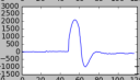
During the course of my physics labwork, a curious problem occurred with our electronics: when the signal too strong, the capacitors inside our digitizes couldn’t handle it. Rather than store the maximum value they basically discharged and reported the ‘maximum’ negative value. Graphically, it looks like this:
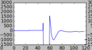
This is obviously a problem. Where there should be a pulse or some sort of other shape, we’ve got a canyon. So how do you fix it? There are a couple of options, but today I’m going to cover the one I’ve explored: interpolation and splines.
What is a spline? Here’s wikipedia’s answer:
…a spline is a numeric function that is piecewise-defined by polynomial functions, and which possesses a high degree of smoothness at the places where the polynomial pieces connect (which are known as knots).[1][2]
In interpolation problems, spline interpolation is often preferred to polynomial interpolation because it yields similar results to interpolating with higher degree polynomials while avoiding instability due to Runge’s phenomenon.
OK, so how does that help us? Basically, it means we can fill in the blanks and ‘fix’ the data given the information we have. The fix won’t be perfect, but in many cases it’s better than nothing. Of course, the stupidest (and simplest) solution in this case might be filling in the blanks with some default value like so:
voltages = []
def pushbackVoltage(V):
   if V < -1800:
      voltages.append(1800)
   else:
      voltages.append(V)
This gives results that look like this:
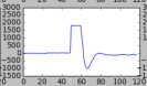
It’s definitely better and would work if you were trying to fix a horizontal line, but not really going to work for any sort of actual data analysis. So we need to do better. Python and matplotlib come to the rescue with several options.
interp1d() and Akima1dInterpolator():
Python’s matplotlib has a function called interp1d. Essentially, you trim out the bad values (or find the spots where your ‘y’ values are missing) then have this function repair your data and fill in the blanks. For my pulses, where I have times and Voltages, it works a little like this:
def pushbackVoltage(self, V):
	if V < -1800:
		self.overflow += 1
		self.times.append(time_increment)
		self.overflowIndices.append(len(self.voltages))
		if splining == 1:
			self.voltages.append(-9000)
		elif flatten_overflow == 1:
			self.voltages.append(1800)
		else:
			self.voltages.append(V)
	else:
		self.times.append(time_increment)
		self.voltages.append(V)

def splineCurve(self):

		tempy = np.delete(self.voltages,self.overflowIndices)
		tempx = np.delete(self.times,self.overflowIndices)
		nearby_voltages = []
		nearby_times = []
		for i in range(-1,0):	#append one voltages, times before the gap
			index = self.overflowIndices[0]+i
			tempV = self.voltages[index]
			nearby_voltages.append(tempV)
			nearby_times.append(self.times[index])
		for i in range(1,5):	#append three voltages, times after the gap
			index = self.overflowIndices[len(self.overflowIndices)-1]+i
			tempV = self.voltages[index]
			nearby_voltages.append(tempV)
			nearby_times.append(self.times[index])

		f = interp1d(nearby_times, nearby_voltages, kind=3)
		#f = Akima1DInterpolator(nearby_times, nearby_voltages)
		for i in range(0,len(self.overflowIndices)):
			index = self.overflowIndices[i]
			self.voltages[index] = f(self.times[index])
What’s going on here?
Basically, two things. First, in my ‘pushbackVoltages()’ function, I store the Voltage array indices where the overflow happens. Then, I add options to check if I want to just flatten the hole, spline it (dump a temporary bad value in there, or ‘nan’), or leave it be.
Next, I call the splineCurve function on all the data. What does it do?
- Deletes whatever is in the offending parts of the voltage array using np.delete. We’re going to fill these in with splined V’s soon.
- Stores voltages and times from before and after the hole in temporary arrays.
- Creates a function to cover the gap, either using interp1d or akima1dinterpolator.
Note here, the options in interp1d. The third option is the type of spline. I chose 3, for a cubical polynomial (think x^3) which works well in my data. You could choose 2 for a parabola, or 1 for a straight line. Below, I’ll show the outputs. There are four, in this order:
- 3d spline (cubic)
- 2d spline (quadratic)
- Akima spline
- 1d spline (linear)
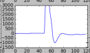
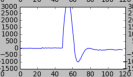
It’s debatable, of course, which one is best, but in this case I think either the cubic or the quadratic got it best. So there we have it! From here, it’s a matter of trying to improve things further. Then, we deal with every coder / analysts nightmare, the endless edge cases.